Code outputs

Stellar evolution and oscillation programs provide their output quantities (e.g. luminosity as a function of age or tables of mode frequencies) in a number of formats. tomso provides functions to make it easier to work with this data.

Most of the loading functions will interpret filenames starting with http as URLs and filenames ending with .gz as gzipped and open them accordingly.

MESA and GYRE

MESA’s histories and profiles and GYRE’s summaries and mode outputs mostly follow a simple text format that can quite easily be read in by NumPy’s genfromtxt function. Each has a set of scalar quantities that are fixed for a given output file (e.g. the effective temperature of a MESA profile or the frequency of a GYRE mode) and a set of columns for quantities that vary, either over a star’s evolution, as a function of position in the star, or, for tables of mode frequencies, as a function of the radial order and angular degree.

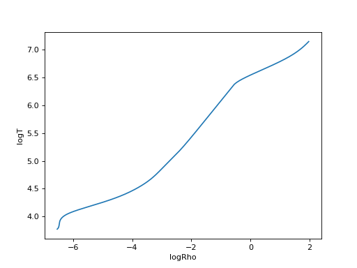
tomso’s functions for reading these files return objects that can be accessed by keys. e.g. to plot logRho against logT,

import matplotlib.pyplot as pl
from tomso.mesa import load_profile
profile = load_profile('../tests/data/mesa.profile')
pl.plot(profile['logRho'], profile['logT'])
pl.xlabel('logRho')
pl.ylabel('logT')

Note that brackets are stripped so in GYRE files, things like Re(freq) become Refreq.

The objects for MESA output files also try to make up for logarithmic keys being absent even if the non-logarithmic form is present (and vice versa). e.g. you could also access T with profile['T'] even if T is absent, as long as logT (or log_T) is. Conversely, you can access logT if T is present but logT isn’t. e.g.:

pl.loglog(profile['Rho'], profile['T'])

will produce the same plot as the previous example even if Rho and T aren’t columns in the profile data.

ADIPLS

ADIPLS produces most of its output in Fortran binary formats and provides tools to convert these to plain text. tomso provides functions to read the binary files directly into Python. The binary output files for the mode frequencies, eigenfunctions and rotation kernels all have the same basic data for the mode frequencies, which is stored in ADIPLS as the arrays cs. You can retrieve the full list of entries from the dtype defined by tomso.adipls.cs_dtypes. e.g.:

from tomso import adipls
print([name for (name, kind) in adipls.cs_dtypes])

Many of the quantities in the cs arrays are then made available through relevant properties.

STARS

The Cambridge stellar evolution code—STARS—provides two main sets of plain text output: plot and out. tomso provides associated routines.

The plot files contains (a lot of!) fixed-width columns of data in plain-text format. The columns can be accessed using the names defined in stars.plot_dtypes. e.g.:

from tomso import stars
print([name for (name, kind) in stars.plot_dtypes])

stars.load_plot currently just returns a NumPy record array and doesn’t (yet) do anything clever with transforming (non-)logarithmic versions of the columns.

The out files contain a mixture of information, starting with a copy of the original fixed-format input control file. There are then regular “summaries”: tables of some stellar properties and, at some user-defined interval, “profiles” that give the interior properties of the star. stars.load_out reads a files and returns a (summaries, profiles) tuple, where each component contains (most of) the data from the file. 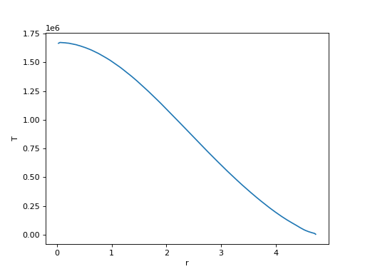The profiles object’s first index is the profile number; the second index is the row number within that model. So you can plot r against T of the last model with something like

import matplotlib.pyplot as pl
from tomso.stars import load_out
summaries, profiles = load_out('../tests/data/stars.out')
pl.plot(profiles[-1]['r'], profiles[-1]['T'])
pl.xlabel('r')
pl.ylabel('T')

The profiles’ columns are defined by the user when they run STARS, so tomso infers their content from the output. You can see what a profile contains with print(profiles.dtype.names).